Consider Again the Example Application of Bayes Rule in Section 6 2 1

Probability based on prior knowledge

"Bayes rule" redirects here. For the concept in decision theory, see Bayes estimator.

A blue neon sign showing the simple statement of Bayes's theorem

In probability theory and statistics, Bayes' theorem (alternatively Bayes' law or Bayes' rule; recently Bayes–Price theorem ^{[i] : 44, 45, 46 and 67} ), named after Thomas Bayes, describes the probability of an event, based on prior knowledge of conditions that might be related to the event.^[2] For example, if the adventure of developing health problems is known to increase with age, Bayes' theorem allows the risk to an private of a known age to be assessed more than accurately (by workout it on their historic period) than simply assuming that the individual is typical of the population as a whole.

One of the many applications of Bayes' theorem is Bayesian inference, a detail arroyo to statistical inference. When applied, the probabilities involved in the theorem may accept different probability interpretations. With Bayesian probability interpretation, the theorem expresses how a degree of belief, expressed as a probability, should rationally change to account for the availability of related show. Bayesian inference is cardinal to Bayesian statistics.

Statement of theorem [edit]

Bayes' theorem is stated mathematically every bit the following equation:^[iii]

${\displaystyle P(A\mid B)={\frac {P(B\mid A)P(A)}{P(B)}}}$

where ${\displaystyle A}$ and ${\displaystyle B}$ are events and ${\displaystyle P(B)\neq 0}$ .

Proof [edit]

For events [edit]

Bayes' theorem may exist derived from the definition of conditional probability:

${\displaystyle P(A\mid B)={\frac {P(A\cap B)}{P(B)}},{\text{ if }}P(B)\neq 0,}$

where ${\displaystyle P(A\cap B)}$ is the probability of both A and B existence truthful. Similarly,

${\displaystyle P(B\mid A)={\frac {P(A\cap B)}{P(A)}},{\text{ if }}P(A)\neq 0,}$

Solving for ${\displaystyle P(A\cap B)}$ and substituting into the above expression for ${\displaystyle P(A\mid B)}$ yields Bayes' theorem:

${\displaystyle P(A\mid B)={\frac {P(B\mid A)P(A)}{P(B)}},{\text{ if }}P(B)\neq 0.}$

For continuous random variables [edit]

For two continuous random variables X and Y, Bayes' theorem may exist analogously derived from the definition of conditional density:

${\displaystyle f_{X\mid Y=y}(x)={\frac {f_{X,Y}(x,y)}{f_{Y}(y)}}}$

${\displaystyle f_{Y\mid X=x}(y)={\frac {f_{X,Y}(x,y)}{f_{X}(x)}}}$

Therefore,

${\displaystyle f_{X\mid Y=y}(x)={\frac {f_{Y\mid X=x}(y)f_{X}(x)}{f_{Y}(y)}}.}$

Examples [edit]

Recreational mathematics [edit]

Bayes' rule and computing conditional probabilities provide a solution method for a number of popular puzzles, such as the Three Prisoners trouble, the Monty Hall trouble, the Two Child problem and the Two Envelopes problem.

Drug testing [edit]

Figure 1: Using a frequency box to show ${\displaystyle P({\text{User}}\mid {\text{Positive}})}$ visually by comparison of shaded areas

Suppose, a item examination for whether someone has been using cannabis is 90% sensitive, significant the true positive rate (TPR)=0.90. Therefore it leads to xc% truthful positive results (correct identification of drug employ) for cannabis users.

The exam is likewise 80% specific, significant truthful negative rate (TNR)=0.lxxx. Therefore the test correctly identifies 80% of non-employ for non-users, but also generates twenty% false positives, or false positive rate (FPR)=0.twenty, for non-users.

Assuming 0.05 prevalence, meaning 5% of people use cannabis, what is the probability that a random person who tests positive is actually a cannabis user?

The Positive predictive value (PPV) of a test is the proportion of persons who are actually positive out of all those testing positive, and tin be calculated from a sample as:

PPV = Truthful positive / Tested positive

If sensitivity, specificity, and prevalence are known, PPV can be calculated using Bayes theorem. Let ${\displaystyle P({\text{User}}\mid {\text{Positive}})}$ mean "the probability that someone is a cannabis user given that they test positive," which is what is meant past PPV. Nosotros tin can write:

${\displaystyle {\begin{aligned}P({\text{User}}\mid {\text{Positive}})&={\frac {P({\text{Positive}}\mid {\text{User}})P({\text{User}})}{P({\text{Positive}})}}\\&={\frac {P({\text{Positive}}\mid {\text{User}})P({\text{User}})}{P({\text{Positive}}\mid {\text{User}})P({\text{User}})+P({\text{Positive}}\mid {\text{Non-user}})P({\text{Non-user}})}}\\[8pt]&={\frac {0.90\times 0.05}{0.90\times 0.05+0.20\times 0.95}}={\frac {0.045}{0.045+0.xix}}\approx 19\%\end{aligned}}}$

The fact that ${\displaystyle P({\text{Positive}})=P({\text{Positive}}\mid {\text{User}})P({\text{User}})+P({\text{Positive}}\mid {\text{Non-user}})P({\text{Not-user}})}$ is a direct application of the Police of Total Probability. In this example, it says that the probability that someone tests positive is the probability that a user tests positive, times the probability of being a user, plus the probability that a non-user tests positive, times the probability of beingness a non-user. This is true because the classifications user and not-user form a partition of a ready, namely the set of people who accept the drug examination. This combined with the definition of conditional probability results in the above statement.

In other words, even if someone tests positive, the probability that they are a cannabis user is merely 19% — this is because in this group, merely five% of people are users, and well-nigh positives are fake positives coming from the remaining 95%.

If i,000 people were tested:

• 950 are not-users and 190 of them requite simulated positive (0.20 × 950)
• fifty of them are users and 45 of them give true positive (0.ninety × fifty)

The i,000 people thus yields 235 positive tests, of which only 45 are 18-carat drug users, about 19%. See Figure 1 for an illustration using a frequency box, and note how pocket-sized the pink area of true positives is compared to the bluish area of false positives.

Sensitivity or specificity [edit]

The importance of specificity can be seen by showing that fifty-fifty if sensitivity is raised to 100% and specificity remains at 80%, the probability of someone testing positive really being a cannabis user but rises from 19% to 21%, but if the sensitivity is held at ninety% and the specificity is increased to 95%, the probability rises to 49%.

Test Actual	Positive	Negative		Total
User	45	v		50
Non-user	190	760		950
Full	235	765	1000
ninety% sensitive, lxxx% specific, PPV=45/235 ≈ 19%

Test Actual	Positive	Negative		Full
User	fifty	0		50
Non-user	190	760		950
Full	240	760	1000
100% sensitive, 80% specific, PPV=l/240 ≈ 21%

Examination Actual	Positive	Negative		Total
User	45	5		fifty
Non-user	47	903		950
Total	92	908	1000
90% sensitive, 95% specific, PPV=45/92 ≈ 49%

Cancer rate [edit]

Even if 100% of patients with pancreatic cancer have a certain symptom, when someone has the same symptom, it does not mean that this person has a 100% gamble of getting pancreatic cancer. Bold the incidence rate of pancreatic cancer is i/100000, while 10/99999 healthy individuals have the same symptoms worldwide, the probability of having pancreatic cancer given the symptoms is only ix.1%, and the other 90.9% could be "false positives" (that is, falsely said to have cancer; "positive" is a disruptive term when, every bit here, the test gives bad news).

Based on incidence rate, the following table presents the corresponding numbers per 100,000 people.

Symptom Cancer	Yes	No		Total
Aye	1	0		one
No	10	99989		99999
Full	eleven	99989	100000

Which can and then be used to calculate the probability of having cancer when you have the symptoms:

${\displaystyle {\begin{aligned}P({\text{Cancer}}|{\text{Symptoms}})&={\frac {P({\text{Symptoms}}|{\text{Cancer}})P({\text{Cancer}})}{P({\text{Symptoms}})}}\\&={\frac {P({\text{Symptoms}}|{\text{Cancer}})P({\text{Cancer}})}{P({\text{Symptoms}}|{\text{Cancer}})P({\text{Cancer}})+P({\text{Symptoms}}|{\text{Not-Cancer}})P({\text{Non-Cancer}})}}\\[8pt]&={\frac {one\times 0.00001}{1\times 0.00001+(10/99999)\times 0.99999}}={\frac {1}{11}}\approx 9.1\%\end{aligned}}}$

Lacking item rate [edit]

Condition Automobile	Lacking	Flawless		Total
A	10	190		200
B	ix	291		300
C	five	495		500
Total	24	976	one thousand

A mill produces an particular using three machines—A, B, and C—which account for xx%, xxx%, and 50% of its output, respectively. Of the items produced past machine A, 5% are defective; similarly, 3% of machine B's items and ane% of machine C'south are defective. If a randomly selected detail is defective, what is the probability information technology was produced by auto C?

Over again, the answer can be reached without using the formula by applying the conditions to a hypothetical number of cases. For example, if the factory produces 1,000 items, 200 volition be produced past Auto A, 300 by Auto B, and 500 past Auto C. Car A will produce 5% × 200 = x defective items, Machine B iii% × 300 = ix, and Motorcar C 1% × 500 = 5, for a total of 24. Thus, the likelihood that a randomly selected defective item was produced by machine C is 5/24 (~20.83%).

This problem can besides exist solved using Bayes' theorem: Let X_i denote the event that a randomly called item was fabricated by the i ^th car (for i = A,B,C). Allow Y denote the event that a randomly called detail is defective. Then, we are given the following information:

${\displaystyle P(X_{A})=0.2,\quad P(X_{B})=0.3,\quad P(X_{C})=0.5.}$

If the item was made by the starting time machine, then the probability that it is defective is 0.05; that is, P(Y |X _A) = 0.05. Overall, nosotros have

${\displaystyle P(Y|X_{A})=0.05,\quad P(Y|X_{B})=0.03,\quad P(Y|X_{C})=0.01.}$

To answer the original question, we first find P(Y). That tin be done in the post-obit way:

${\displaystyle P(Y)=\sum _{i}P(Y|X_{i})P(X_{i})=(0.05)(0.ii)+(0.03)(0.3)+(0.01)(0.5)=0.024.}$

Hence, two.4% of the total output is defective.

We are given that Y has occurred, and we want to calculate the conditional probability of X _C. By Bayes' theorem,

${\displaystyle P(X_{C}|Y)={\frac {P(Y|X_{C})P(X_{C})}{P(Y)}}={\frac {0.01\cdot 0.50}{0.024}}={\frac {five}{24}}}$

Given that the detail is defective, the probability that it was made past automobile C is 5/24. Although car C produces half of the total output, it produces a much smaller fraction of the defective items. Hence the knowledge that the item selected was defective enables us to replace the prior probability P(10 _C) = 1/two by the smaller posterior probability P(X_C |Y) = 5/24.

Interpretations [edit]

Figure 2: A geometric visualisation of Bayes' theorem.

The estimation of Bayes' dominion depends on the estimation of probability ascribed to the terms. The two main interpretations are described below. Figure 2 shows a geometric visualization similar to Figure i. Gerd Gigerenzer and co-authors take pushed hard for educational activity Bayes Rule this way, with special accent on teaching it to physicians.^[4] An example is Volition Kurt'southward webpage, "Bayes' Theorem with Lego," after turned into the book, Bayesian Statistics the Fun Way: Understanding Statistics and Probability with Star Wars, LEGO, and Rubber Ducks. Zhu and Gigerenzer found in 2006 that whereas 0% of quaternary, 5th, and 6th-graders could solve give-and-take problems after beingness taught with formulas, 19%, 39%, and 53% could subsequently being taught with frequency boxes, and that the learning was either thorough or zero.^[5]

Bayesian estimation [edit]

In the Bayesian (or epistemological) interpretation, probability measures a "degree of belief". Bayes' theorem links the degree of belief in a proffer before and after accounting for show. For example, suppose it is believed with 50% certainty that a coin is twice as likely to land heads than tails. If the coin is flipped a number of times and the outcomes observed, that degree of belief will probably rise or fall, but might even remain the same, depending on the results. For proposition A and evidence B,

• P (A), the prior, is the initial degree of belief in A.
• P (A |B), the posterior, is the degree of belief after incorporating news that B is true.
• the quotient P(B |A) / P(B) represents the support B provides for A.

For more on the application of Bayes' theorem under the Bayesian interpretation of probability, see Bayesian inference.

Frequentist interpretation [edit]

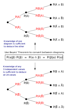
Figure 3: Illustration of frequentist interpretation with tree diagrams.

In the frequentist estimation, probability measures a "proportion of outcomes". For example, suppose an experiment is performed many times. P(A) is the proportion of outcomes with holding A (the prior) and P(B) is the proportion with property B. P(B |A) is the proportion of outcomes with belongings B out of outcomes with property A, and P(A |B) is the proportion of those with A out of those withB (the posterior).

The office of Bayes' theorem is all-time visualized with tree diagrams such every bit Figure 3. The two diagrams partition the same outcomes by A and B in opposite orders, to obtain the inverse probabilities. Bayes' theorem links the unlike partitionings.

Example [edit]

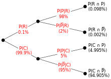
Figure four: Tree diagram illustrating the protrude example. R, C, P and ${\displaystyle {\overline {P}}}$ are the events rare, common, pattern and no pattern. Percentages in parentheses are calculated. Three independent values are given, so it is possible to calculate the inverse tree.

An entomologist spots what might, due to the pattern on its back, be a rare subspecies of protrude. A full 98% of the members of the rare subspecies have the pattern, then P(Design | Rare) = 98%. Only 5% of members of the common subspecies have the pattern. The rare subspecies is 0.1% of the total population. How likely is the protrude having the design to be rare: what is P(Rare | Pattern)?

From the extended grade of Bayes' theorem (since whatever beetle is either rare or common),

${\displaystyle {\brainstorm{aligned}P({\text{Rare}}\mid {\text{Pattern}})&={\frac {P({\text{Pattern}}\mid {\text{Rare}})P({\text{Rare}})}{P({\text{Blueprint}})}}\\[8pt]&={\frac {P({\text{Design}}\mid {\text{Rare}})P({\text{Rare}})}{P({\text{Pattern}}\mid {\text{Rare}})P({\text{Rare}})+P({\text{Design}}\mid {\text{Common}})P({\text{Common}})}}\\[8pt]&={\frac {0.98\times 0.001}{0.98\times 0.001+0.05\times 0.999}}\\[8pt]&\approx one.9\%\cease{aligned}}}$

Forms [edit]

Events [edit]

Simple form [edit]

For events A and B, provided that P(B) ≠ 0,

${\displaystyle P(A|B)={\frac {P(B|A)P(A)}{P(B)}}\cdot }$

In many applications, for instance in Bayesian inference, the consequence B is stock-still in the discussion, and nosotros wish to consider the impact of its having been observed on our belief in various possible events A. In such a state of affairs the denominator of the terminal expression, the probability of the given prove B, is fixed; what we want to vary is A. Bayes' theorem and so shows that the posterior probabilities are proportional to the numerator, so the final equation becomes:

${\displaystyle P(A|B)\propto P(A)\cdot P(B|A)}$ .

In words, the posterior is proportional to the prior times the likelihood.^{[half dozen]}

If events A ₁, A ₂, ..., are mutually exclusive and exhaustive, i.east., i of them is certain to occur but no two tin can occur together, we tin can determine the proportionality abiding by using the fact that their probabilities must add upward to one. For instance, for a given upshot A, the event A itself and its complement ¬A are exclusive and exhaustive. Denoting the abiding of proportionality by c we accept

${\displaystyle P(A|B)=c\cdot P(A)\cdot P(B|A){\text{ and }}P(\neg A|B)=c\cdot P(\neg A)\cdot P(B|\neg A).}$

Adding these two formulas we deduce that

${\displaystyle 1=c\cdot (P(B|A)\cdot P(A)+P(B|\neg A)\cdot P(\neg A)),}$

or

${\displaystyle c={\frac {1}{P(B|A)\cdot P(A)+P(B|\neg A)\cdot P(\neg A)}}={\frac {1}{P(B)}}.}$

Alternative form [edit]

Contingency tabular array

Background Proposition	B	¬B (non B)		Total
A	P(B|A)·P(A) = P(A|B)·P(B)	P(¬B|A)·P(A) = P(A|¬B)·P(¬B)		P(A)
¬A (not A)	P(B|¬A)·P(¬A) = P(¬A|B)·P(B)	P(¬B|¬A)·P(¬A) = P(¬A|¬B)·P(¬B)		P(¬A) = i−P(A)
Full	P(B)	P(¬B) = 1−P(B)	1

Another form of Bayes' theorem for two competing statements or hypotheses is:

${\displaystyle P(A|B)={\frac {P(B|A)P(A)}{P(B|A)P(A)+P(B|\neg A)P(\neg A)}}.}$

For an epistemological interpretation:

For suggestion A and evidence or background B,^[vii]

Extended course [edit]

Often, for some sectionalisation {A_j } of the sample infinite, the event space is given in terms of P(A_j ) and P(B |A_j ). It is then useful to compute P(B) using the law of total probability:

${\displaystyle P(B)={\sum _{j}P(B|A_{j})P(A_{j})},}$

${\displaystyle \Rightarrow P(A_{i}|B)={\frac {P(B|A_{i})P(A_{i})}{\sum \limits _{j}P(B|A_{j})P(A_{j})}}\cdot }$

In the special instance where A is a binary variable:

${\displaystyle P(A|B)={\frac {P(B|A)P(A)}{P(B|A)P(A)+P(B|\neg A)P(\neg A)}}\cdot }$

Random variables [edit]

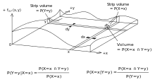
Figure v: Bayes' theorem applied to an event space generated by continuous random variables X and Y. There exists an instance of Bayes' theorem for each point in the domain. In practice, these instances might be parametrized by writing the specified probability densities as a function of x and y.

Consider a sample space Ω generated by two random variables 10 and Y. In principle, Bayes' theorem applies to the events A = {Ten =ten} and B = {Y =y}.

${\displaystyle P(10{=}x|Y{=}y)={\frac {P(Y{=}y|X{=}ten)P(X{=}x)}{P(Y{=}y)}}}$

However, terms go 0 at points where either variable has finite probability density. To remain useful, Bayes' theorem must be formulated in terms of the relevant densities (see Derivation).

Simple form [edit]

If Ten is continuous and Y is discrete,

${\displaystyle f_{Ten|Y{=}y}(10)={\frac {P(Y{=}y|X{=}x)f_{Ten}(x)}{P(Y{=}y)}}}$

where each ${\displaystyle f}$ is a density part.

If X is discrete and Y is continuous,

${\displaystyle P(10{=}x|Y{=}y)={\frac {f_{Y|X{=}10}(y)P(Ten{=}10)}{f_{Y}(y)}}.}$

If both X and Y are continuous,

${\displaystyle f_{X|Y{=}y}(x)={\frac {f_{Y|X{=}x}(y)f_{X}(x)}{f_{Y}(y)}}.}$

Extended grade [edit]

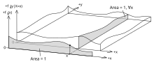
Effigy 6: A fashion to conceptualize event spaces generated by continuous random variables Ten and Y.

A continuous event space is frequently conceptualized in terms of the numerator terms. It is so useful to eliminate the denominator using the law of total probability. For f_Y (y), this becomes an integral:

${\displaystyle f_{Y}(y)=\int _{-\infty }^{\infty }f_{Y|X=\xi }(y)f_{X}(\11 )\,d\xi .}$

Bayes' rule in odds form [edit]

Bayes' theorem in odds class is:

${\displaystyle O(A_{1}:A_{ii}\mid B)=O(A_{1}:A_{2})\cdot \Lambda (A_{i}:A_{two}\mid B)}$

where

${\displaystyle \Lambda (A_{one}:A_{ii}\mid B)={\frac {P(B\mid A_{1})}{P(B\mid A_{2})}}}$

is called the Bayes gene or likelihood ratio. The odds between two events is simply the ratio of the probabilities of the two events. Thus

${\displaystyle O(A_{i}:A_{two})={\frac {P(A_{i})}{P(A_{2})}},}$

${\displaystyle O(A_{ane}:A_{2}\mid B)={\frac {P(A_{1}\mid B)}{P(A_{2}\mid B)}},}$

Thus, the rule says that the posterior odds are the prior odds times the Bayes cistron, or in other words, the posterior is proportional to the prior times the likelihood.

In the special case that ${\displaystyle A_{1}=A}$ and ${\displaystyle A_{2}=\neg A}$ , ane writes ${\displaystyle O(A)=O(A:\neg A)=P(A)/(1-P(A))}$ , and uses a similar abbreviation for the Bayes factor and for the provisional odds. The odds on ${\displaystyle A}$ is by definition the odds for and against ${\displaystyle A}$ . Bayes' rule tin so be written in the abbreviated form

${\displaystyle O(A\mid B)=O(A)\cdot \Lambda (A\mid B),}$

or, in words, the posterior odds on ${\displaystyle A}$ equals the prior odds on ${\displaystyle A}$ times the likelihood ratio for ${\displaystyle A}$ given data ${\displaystyle B}$ . In short, posterior odds equals prior odds times likelihood ratio.

For instance, if a medical test has a sensitivity of 90% and a specificity of 91%, then the positive Bayes factor is ${\displaystyle \Lambda _{+}=P({\text{True Positive}})/P({\text{Imitation Positive}})=90\%/(100\%-91\%)=10}$ . At present, if the prevalence of this affliction is 9.09%, and if we take that as the prior probability, then the prior odds is about ane:10. So afterwards receiving a positive exam result, the posterior odds of actually having the disease becomes i:1; In other words, the posterior probability of actually having the disease is 50%. If a second test is performed in serial testing, and that also turns out to be positive, then the posterior odds of actually having the disease becomes 10:1, which means a posterior probability of about ninety.91%. The negative Bayes cistron tin can exist calculated to exist 91%/(100%-90%)=9.1, so if the 2nd examination turns out to be negative, so the posterior odds of actually having the illness is ane:9.i, which means a posterior probability of about 9.9%.

The example above tin too be understood with more than solid numbers: Assume the patient taking the exam is from a group of 1000 people, where 91 of them actually have the disease (prevalence of 9.1%). If all these 1000 people have the medical test, 82 of those with the disease will get a true positive issue (sensitivity of 90.one%), 9 of those with the disease volition get a faux negative upshot (false negative rate of 9.9%), 827 of those without the disease will get a true negative result (specificivity of 91.0%), and 82 of those without the affliction will get a simulated positive result (imitation positive rate of ix.0%). Before taking whatever examination, the patient'southward odds for having the affliction is 91:909. Afterward receiving a positive result, the patient's odds for having the disease is

${\displaystyle {\frac {91}{909}}\times {\frac {90.ane\%}{ix.0\%}}={\frac {91\times 90.1\%}{909\times nine.0\%}}=1:1}$

which is consistent with the fact that at that place are 82 true positives and 82 false positives in the group of g people.

Correspondence to other mathematical frameworks [edit]

Propositional logic [edit]

Using ${\displaystyle P(\neg B\mid A)=one-P(B\mid A)}$ twice, one may use Bayes' theorem to too express ${\displaystyle P(\neg B\mid \neg A)}$ in terms of ${\displaystyle P(A\mid B)}$ and without negations:

${\displaystyle P(\neg B\mid \neg A)=1-\left(1-P(A\mid B)\right){\frac {P(B)}{P(\neg A)}}}$ ,

when ${\displaystyle P(\neg A)=1-P(A)\neq 0}$ . From this we tin read off the inference

${\displaystyle P(A\mid B)=i\implies P(\neg B\mid \neg A)=1}$ .

In words: If certainly ${\displaystyle B}$ implies ${\displaystyle A}$ , we infer that certainly ${\displaystyle \neg A}$ implies ${\displaystyle \neg B}$ . Where ${\displaystyle P(B)\neq 0}$ , the two implications beingness certain are equivalent statements. In the probability formulas, the conditional probability ${\displaystyle P(A\mid B)}$ generalizes the logical implication ${\displaystyle B\implies A}$ , where at present beyond assigning true or false, we assign probability values to statements. The assertion of ${\displaystyle B\implies A}$ is captured past certainty of the conditional, the assertion of ${\displaystyle P(A\mid B)=ane}$ . Relating the directions of implication, Bayes' theorem represents a generalization of the contraposition constabulary, which in classical propositional logic can be expressed as:

${\displaystyle (B\implies A)\iff (\neg A\implies \neg B)}$ .

Note that in this relation between implications, the positions of ${\displaystyle A}$ resp. ${\displaystyle B}$ go flipped.

The respective formula in terms of probability calculus is Bayes' theorem, which in its expanded form involving the prior probability/base charge per unit ${\displaystyle a}$ of only ${\displaystyle A}$ , is expressed as:^[viii]

${\displaystyle P(A\mid B)=P(B\mid A){\frac {a(A)}{P(B\mid A)\,a(A)+P(B\mid \neg A)\,a(\neg A)}}}$ .

Subjective logic [edit]

Bayes' theorem represents a special case of deriving inverted provisional opinions in subjective logic expressed as:

${\displaystyle (\omega _{A{\tilde {|}}B}^{Due south},\omega _{A{\tilde {|}}\lnot B}^{S})=(\omega _{B\mid A}^{S},\omega _{B\mid \lnot A}^{Southward}){\widetilde {\phi }}a_{A},}$

where ${\displaystyle {\widetilde {\phi }}}$ denotes the operator for inverting conditional opinions. The statement ${\displaystyle (\omega _{B\mid A}^{South},\omega _{B\mid \lnot A}^{Due south})}$ denotes a pair of binomial conditional opinions given past source ${\displaystyle Due south}$ , and the argument ${\displaystyle a_{A}}$ denotes the prior probability (aka. the base rate) of ${\displaystyle A}$ . The pair of derivative inverted conditional opinions is denoted ${\displaystyle (\omega _{A{\tilde {|}}B}^{S},\omega _{A{\tilde {|}}\lnot B}^{South})}$ . The conditional opinion ${\displaystyle \omega _{A\mid B}^{Southward}}$ generalizes the probabilistic conditional ${\displaystyle P(A\mid B)}$ , i.e. in addition to assigning a probability the source ${\displaystyle Due south}$ tin assign any subjective opinion to the conditional statement ${\displaystyle (A\mid B)}$ . A binomial subjective stance ${\displaystyle \omega _{A}^{S}}$ is the belief in the truth of statement ${\displaystyle A}$ with degrees of epistemic uncertainty, as expressed past source ${\displaystyle S}$ . Every subjective opinion has a corresponding projected probability ${\displaystyle P(\omega _{A}^{S})}$ . The application of Bayes' theorem to projected probabilities of opinions is a homomorphism, significant that Bayes' theorem tin exist expressed in terms of projected probabilities of opinions:

${\displaystyle P(\omega _{A{\tilde {|}}B}^{S})={\frac {P(\omega _{B\mid A}^{S})a(A)}{P(\omega _{B\mid A}^{Due south})a(A)+P(\omega _{B\mid \lnot A}^{South})a(\lnot A)}}.}$

Hence, the subjective Bayes' theorem represents a generalization of Bayes' theorem.^[nine]

Generalizations [edit]

Conditioned version [edit]

A conditioned version of the Bayes' theorem^[10] results from the addition of a third outcome ${\displaystyle C}$ on which all probabilities are conditioned:

${\displaystyle P(A\mid B\cap C)={\frac {P(B\mid A\cap C)\,P(A\mid C)}{P(B\mid C)}}}$

Derivation [edit]

Using the chain rule

${\displaystyle P(A\cap B\cap C)=P(A\mid B\cap C)\,P(B\mid C)\,P(C)}$

And, on the other manus

${\displaystyle P(A\cap B\cap C)=P(B\cap A\cap C)=P(B\mid A\cap C)\,P(A\mid C)\,P(C)}$

The desired result is obtained by identifying both expressions and solving for ${\displaystyle P(A\mid B\cap C)}$ .

Bayes' rule with 3 events [edit]

In the case of 3 events - A, B, and C - information technology tin be shown that:

$${\displaystyle P(A\mid B,C)={\frac {P(B\mid A,C)\;P(A\mid C)}{P(B\mid C)}}}$$

Proof^[11]

$${\displaystyle {\begin{aligned}P(A\mid B,C)&={\frac {P(A,B,C)}{P(B,C)}}\\[1ex]&={\frac {P(B\mid A,C)\,P(A,C)}{P(B,C)}}\\[1ex]&={\frac {P(B\mid A,C)\,P(A\mid C)\,P(C)}{P(B,C)}}\\[1ex]&={\frac {P(B\mid A,C)\,P(A\mid C)P(C)}{P(B\mid C)P(C)}}\\[1ex]&={\frac {P(B\mid A,C)\;P(A\mid C)}{P(B\mid C)}}\end{aligned}}}$$

History [edit]

Bayes' theorem is named afterwards the Reverend Thomas Bayes (; c. 1701 – 1761), who first used conditional probability to provide an algorithm (his Suggestion 9) that uses evidence to summate limits on an unknown parameter, published every bit An Essay towards solving a Problem in the Doctrine of Chances (1763). He studied how to compute a distribution for the probability parameter of a binomial distribution (in modern terminology). On Bayes'south death his family transferred his papers to his old friend, Richard Price (1723–1791) who over a period of two years significantly edited the unpublished manuscript, before sending it to a friend who read it aloud at the Royal Society on 23 December 1763.^{[i] [ page needed ]} Price edited^[12] Bayes'southward major work "An Essay towards solving a Problem in the Doctrine of Chances" (1763), which appeared in Philosophical Transactions,^[13] and contains Bayes' theorem. Price wrote an introduction to the newspaper which provides some of the philosophical basis of Bayesian statistics and chose i of the two solutions offered past Bayes. In 1765, Price was elected a Beau of the Regal Society in recognition of his work on the legacy of Bayes.^{[fourteen] [15]} On 27 April a alphabetic character sent to his friend Benjamin Franklin was read out at the Purple Order, and after published, where Price applies this piece of work to population and computing 'life-annuities'.^[xvi]

Independently of Bayes, Pierre-Simon Laplace in 1774, and later in his 1812 Théorie analytique des probabilités, used conditional probability to formulate the relation of an updated posterior probability from a prior probability, given evidence. He reproduced and extended Bayes's results in 1774, apparently unaware of Bayes's work.^{[note 1] [17]} The Bayesian interpretation of probability was adult mainly by Laplace.^[18]

Sir Harold Jeffreys put Bayes's algorithm and Laplace'due south formulation on an evident basis, writing that Bayes' theorem "is to the theory of probability what the Pythagorean theorem is to geometry".^[19]

Stephen Stigler used a Bayesian argument to conclude that Bayes' theorem was discovered by Nicholas Saunderson, a blind English mathematician, some time before Bayes;^{[20] [21]} that estimation, nonetheless, has been disputed.^[22] Martyn Hooper^[23] and Sharon McGrayne^[24] take argued that Richard Price'south contribution was substantial:

By modern standards, we should refer to the Bayes–Price rule. Price discovered Bayes's work, recognized its importance, corrected it, contributed to the commodity, and found a use for it. The modern convention of employing Bayes'south proper noun alone is unfair but so entrenched that anything else makes little sense.^[24]

Apply in genetics [edit]

In genetics, Bayes' theorem can exist used to summate the probability of an individual having a specific genotype. Many people seek to approximate their chances of being affected by a genetic disease or their likelihood of being a carrier for a recessive gene of interest. A Bayesian analysis can be done based on family history or genetic testing, in order to predict whether an individual volition develop a illness or pass one on to their children. Genetic testing and prediction is a common practice among couples who plan to have children merely are concerned that they may both be carriers for a illness, especially within communities with low genetic variance.^[25]

The outset step in Bayesian analysis for genetics is to propose mutually exclusive hypotheses: for a specific allele, an individual either is or is not a carrier. Next, four probabilities are calculated: Prior Probability (the likelihood of each hypothesis considering information such equally family unit history or predictions based on Mendelian Inheritance), Conditional Probability (of a certain outcome), Joint Probability (production of the first two), and Posterior Probability (a weighted product calculated past dividing the Articulation Probability for each hypothesis by the sum of both joint probabilities). This type of analysis can be done based purely on family history of a condition or in concert with genetic testing.^{[ citation needed ]}

Using pedigree to calculate probabilities [edit]

Hypothesis	Hypothesis 1: Patient is a carrier	Hypothesis 2: Patient is non a carrier
Prior Probability	ane/2	ane/ii
Conditional Probability that all four offspring volition be unaffected	(ane/2) · (1/2) · (1/2) · (ane/2) = 1/16	Well-nigh ane
Joint Probability	(1/2) · (i/xvi) = 1/32	(1/2) · ane = i/2
Posterior Probability	(one/32) / (1/32 + one/2) = 1/17	(ane/two) / (1/32 + 1/2) = 16/17

Example of a Bayesian assay tabular array for a female individual'south risk for a illness based on the noesis that the disease is present in her siblings merely not in her parents or whatsoever of her iv children. Based solely on the status of the subject's siblings and parents, she is equally likely to be a carrier every bit to be a non-carrier (this likelihood is denoted by the Prior Hypothesis). However, the probability that the subject's four sons would all exist unaffected is 1/16 (½·½·½·½) if she is a carrier, about 1 if she is a non-carrier (this is the Provisional Probability). The Articulation Probability reconciles these two predictions by multiplying them together. The last line (the Posterior Probability) is calculated past dividing the Articulation Probability for each hypothesis by the sum of both articulation probabilities.^[26]

Using genetic examination results [edit]

Parental genetic testing can detect effectually ninety% of known disease alleles in parents that can lead to carrier or affected status in their child. Cystic fibrosis is a heritable disease caused by an autosomal recessive mutation on the CFTR gene,^[27] located on the q arm of chromosome vii.^[28]

Bayesian analysis of a female patient with a family history of cystic fibrosis (CF), who has tested negative for CF, demonstrating how this method was used to determine her take a chance of having a child born with CF:

Because the patient is unaffected, she is either homozygous for the wild-blazon allele, or heterozygous. To establish prior probabilities, a Punnett foursquare is used, based on the knowledge that neither parent was afflicted by the affliction just both could have been carriers:

Mother Male parent	Westward Homozygous for the wild- type allele (a not-carrier)	M Heterozygous (a CF carrier)
W Homozygous for the wild- type allele (a non-carrier)	WW	MW
M Heterozygous (a CF carrier)	MW	MM (afflicted by cystic fibrosis)

Given that the patient is unaffected, at that place are only 3 possibilities. Inside these three, there are ii scenarios in which the patient carries the mutant allele. Thus the prior probabilities are ⅔ and ⅓.

Next, the patient undergoes genetic testing and tests negative for cystic fibrosis. This test has a xc% detection rate, so the conditional probabilities of a negative test are 1/10 and one.  Finally, the joint and posterior probabilities are calculated equally earlier.

Hypothesis	Hypothesis 1: Patient is a carrier	Hypothesis 2: Patient is not a carrier
Prior Probability	2/3	1/three
Provisional Probability of a negative test	1/10	1
Articulation Probability	1/15	1/3
Posterior Probability	one/half dozen	5/6

After carrying out the same analysis on the patient'due south male person partner (with a negative test result), the chances of their child being affected is equal to the product of the parents' respective posterior probabilities for existence carriers times the chances that ii carriers will produce an afflicted offspring (¼).

Genetic testing done in parallel with other risk factor identification. [edit]

Bayesian analysis tin exist done using phenotypic information associated with a genetic status, and when combined with genetic testing this assay becomes much more complicated. Cystic Fibrosis, for case, can be identified in a fetus through an ultrasound looking for an echogenic bowel, meaning one that appears brighter than normal on a scan2. This is not a foolproof exam, equally an echogenic bowel can be nowadays in a  perfectly good for you fetus. Parental genetic testing is very influential in this case, where a phenotypic facet can be overly influential in probability calculation. In the case of a fetus with an echogenic bowel, with a mother who has been tested and is known to be a CF carrier, the posterior probability that the fetus really has the illness is very high (0.64). All the same, once the father has tested negative for CF, the posterior probability drops significantly (to 0.16).^[26]

Risk factor adding is a powerful tool in genetic counseling and reproductive planning, but it cannot exist treated as the only important factor to consider. As higher up, incomplete testing can yield falsely high probability of carrier condition, and testing tin exist financially inaccessible or unfeasible when a parent is non present.

See also [edit]

• Bayesian epistemology
• Inductive probability
• Quantum Bayesianism
• Why Most Published Research Findings Are False, a 2005 essay in metascience by John Ioannidis

Notes [edit]

1. ^ Laplace refined Bayes's theorem over a period of decades:
   • Laplace announced his independent discovery of Bayes' theorem in: Laplace (1774) "Mémoire sur la probabilité des causes par les événements," "Mémoires de l'Académie royale des Sciences de MI (Savants étrangers)," 4: 621–656. Reprinted in: Laplace, "Oeuvres complètes" (Paris, French republic: Gauthier-Villars et fils, 1841), vol. 8, pp. 27–65. Bachelor on-line at: Gallica. Bayes' theorem appears on p. 29.
   • Laplace presented a refinement of Bayes' theorem in: Laplace (read: 1783 / published: 1785) "Mémoire sur les approximations des formules qui sont fonctions de très grands nombres," "Mémoires de l'Académie royale des Sciences de Paris," 423–467. Reprinted in: Laplace, "Oeuvres complètes" (Paris, France: Gauthier-Villars et fils, 1844), vol. 10, pp. 295–338. Available on-line at: Gallica. Bayes' theorem is stated on page 301.
   • Run into as well: Laplace, "Essai philosophique sur les probabilités" (Paris, France: Mme. Ve. Courcier [Madame veuve (i.e., widow) Courcier], 1814), page ten. English language translation: Pierre Simon, Marquis de Laplace with F. Due west. Truscott and F. L. Emory, trans., "A Philosophical Essay on Probabilities" (New York, New York: John Wiley & Sons, 1902), folio fifteen.

References [edit]

1. ^ ^{a b} Frame, Paul (2015). Liberty'southward Campaigner. Wales: University of Wales Printing. ISBN978-1-78316-216-1 . Retrieved 23 Feb 2021.
2. ^ Joyce, James (2003), "Bayes' Theorem", in Zalta, Edward Northward. (ed.), The Stanford Encyclopedia of Philosophy (Jump 2019 ed.), Metaphysics Research Lab, Stanford University, retrieved 2020-01-17
3. ^ Stuart, A.; Ord, K. (1994), Kendall's Advanced Theory of Statistics: Book I—Distribution Theory, Edward Arnold, §eight.7
4. ^ Gigerenzer, Gerd; Hoffrage, Ulrich (1995). "How to meliorate Bayesian reasoning without instruction: Frequency formats". Psychological Review. 102 (4): 684–704. CiteSeerX10.one.ane.128.3201. doi:x.1037/0033-295X.102.iv.684.
5. ^ Zhu, Liqi; Gigerenzer, Gerd (January 2006). "Children tin solve Bayesian problems: the part of representation in mental computation". Cognition. 98 (3): 287–308. doi:10.1016/j.knowledge.2004.12.003. hdl:11858/00-001M-0000-0024-FEFD-A. PMID 16399266. S2CID 1451338.
6. ^ Lee, Peter M. (2012). "Affiliate 1". Bayesian Statistics. Wiley. ISBN978-1-1183-3257-3.
7. ^ "Bayes' Theorem: Introduction". Trinity Academy. Archived from the original on 21 August 2004. Retrieved 5 August 2014.
8. ^ Audun Jøsang, 2016, Subjective Logic; A formalism for Reasoning Under Uncertainty. Springer, Cham, ISBN 978-iii-319-42337-1
9. ^ Audun Jøsang, 2016, Generalising Bayes' Theorem in Subjective Logic. IEEE International Conference on Multisensor Fusion and Integration for Intelligent Systems (MFI 2016), Baden-Baden, September 2016
10. ^ Koller, D.; Friedman, N. (2009). Probabilistic Graphical Models. Massachusetts: MIT Press. p. 1208. ISBN978-0-262-01319-2. Archived from the original on 2014-04-27.
11. ^ Graham Kemp (https://math.stackexchange.com/users/135106/graham-kemp), Bayes' rule with iii variables, URL (version: 2015-05-14): https://math.stackexchange.com/q/1281558
12. ^ Allen, Richard (1999). David Hartley on Human Nature. SUNY Press. pp. 243–4. ISBN978-0-7914-9451-6 . Retrieved 16 June 2013.
13. ^ Bayes, Thomas & Cost, Richard (1763). "An Essay towards solving a Problem in the Doctrine of Chance. By the late Rev. Mr. Bayes, communicated by Mr. Price, in a letter of the alphabet to John County, A. K. F. R. Southward." Philosophical Transactions of the Royal Society of London. 53: 370–418. doi:10.1098/rstl.1763.0053.
14. ^ Holland, pp. 46–7.
15. ^ Toll, Richard (1991). Price: Political Writings. Cambridge University Press. p. xxiii. ISBN978-0-521-40969-8 . Retrieved 16 June 2013.
16. ^ Mitchell 1911, p. 314 harvnb error: no target: CITEREFMitchell1911 (help).
17. ^ Daston, Lorraine (1988). Classical Probability in the Enlightenment. Princeton Univ Press. p. 268. ISBN0-691-08497-ane.
18. ^ Stigler, Stephen Yard. (1986). "Changed Probability". The History of Statistics: The Measurement of Uncertainty Earlier 1900. Harvard University Press. pp. 99–138. ISBN978-0-674-40341-3.
19. ^ Jeffreys, Harold (1973). Scientific Inference (tertiary ed.). Cambridge University Press. p. 31. ISBN978-0-521-18078-8.
20. ^ Stigler, Stephen Grand. (1983). "Who Discovered Bayes' Theorem?". The American Statistician. 37 (iv): 290–296. doi:x.1080/00031305.1983.10483122.
21. ^ de Vaux, Richard; Velleman, Paul; Bock, David (2016). Stats, Data and Models (quaternary ed.). Pearson. pp. 380–381. ISBN978-0-321-98649-eight.
22. ^ Edwards, A. W. F. (1986). "Is the Reference in Hartley (1749) to Bayesian Inference?". The American Statistician. forty (two): 109–110. doi:10.1080/00031305.1986.10475370.
23. ^ Hooper, Martyn (2013). "Richard Cost, Bayes' theorem, and God". Significance. ten (1): 36–39. doi:10.1111/j.1740-9713.2013.00638.x. S2CID 153704746.
24. ^ ^{a b} McGrayne, S. B. (2011). The Theory That Would Not Die: How Bayes' Dominion Cracked the Enigma Lawmaking, Hunted Down Russian Submarines & Emerged Triumphant from Two Centuries of Controversy . Yale Academy Printing. ISBN978-0-300-18822-6.
25. ^ Kraft, Stephanie A; Duenas, Devan; Wilfond, Benjamin Due south; Goddard, Katrina AB (24 September 2018). "The evolving landscape of expanded carrier screening: challenges and opportunities". Genetics in Medicine. 21 (4): 790–797. doi:x.1038/s41436-018-0273-4. PMC6752283. PMID 30245516.
26. ^ ^{a b} Ogino, Shuji; Wilson, Robert B; Aureate, Bert; Hawley, Pamela; Grody, Wayne W (October 2004). "Bayesian analysis for cystic fibrosis risks in prenatal and carrier screening". Genetics in Medicine. 6 (5): 439–449. doi:x.1097/01.GIM.0000139511.83336.8F. PMID 15371910.
27. ^ "Types of CFTR Mutations". Cystic Fibrosis Foundation, world wide web.cff.org/What-is-CF/Genetics/Types-of-CFTR-Mutations/.
28. ^ "CFTR Cistron – Genetics Home Reference". U.South. National Library of Medicine, National Institutes of Health, ghr.nlm.nih.gov/factor/CFTR#location.

Further reading [edit]

• Grunau, Hans-Christoph (24 January 2014). "Preface Effect 3/4-2013". Jahresbericht der Deutschen Mathematiker-Vereinigung. 115 (three–4): 127–128. doi:10.1365/s13291-013-0077-z.
• Gelman, A, Carlin, JB, Stern, HS, and Rubin, DB (2003), "Bayesian Data Analysis," Second Edition, CRC Press.
• Grinstead, CM and Snell, JL (1997), "Introduction to Probability (second edition)," American Mathematical Social club (free pdf available) [1].
• "Bayes formula", Encyclopedia of Mathematics, Ems Printing, 2001 [1994]
• McGrayne, SB (2011). The Theory That Would Not Die: How Bayes' Rule Cracked the Enigma Code, Hunted Down Russian Submarines & Emerged Triumphant from Ii Centuries of Controversy . Yale Academy Printing. ISBN978-0-300-18822-6.
• Laplace, Pierre Simon (1986). "Memoir on the Probability of the Causes of Events". Statistical Scientific discipline. i (iii): 364–378. doi:x.1214/ss/1177013621. JSTOR 2245476.
• Lee, Peter M (2012), "Bayesian Statistics: An Introduction," quaternary edition. Wiley. ISBN 978-1-118-33257-iii.
• Puga JL, Krzywinski M, Altman Northward (31 March 2015). "Bayes' theorem". Nature Methods. 12 (four): 277–278. doi:x.1038/nmeth.3335. PMID 26005726.
• Rosenthal, Jeffrey S (2005), "Struck by Lightning: The Curious World of Probabilities". HarperCollins. (Granta, 2008. ISBN 9781862079960).
• Stigler, Stephen M. (August 1986). "Laplace'southward 1774 Memoir on Inverse Probability". Statistical Science. ane (3): 359–363. doi:10.1214/ss/1177013620.
• Stone, JV (2013), download chapter one of "Bayes' Rule: A Tutorial Introduction to Bayesian Assay", Sebtel Press, England.
• Bayesian Reasoning for Intelligent People, An introduction and tutorial to the use of Bayes' theorem in statistics and cognitive science.
• Morris, Dan (2016), Read first 6 chapters for free of "Bayes' Theorem Examples: A Visual Introduction For Beginners" Blue Windmill ISBN 978-1549761744. A short tutorial on how to understand problem scenarios and observe P(B), P(A), and P(B|A).

External links [edit]

• Visual explanation of Bayes using trees (video)
• Bayes' frequentist interpretation explained visually (video)
• Earliest Known Uses of Some of the Words of Mathematics (B). Contains origins of "Bayesian", "Bayes' Theorem", "Bayes Estimate/Run a risk/Solution", "Empirical Bayes", and "Bayes Factor".
• A tutorial on probability and Bayes' theorem devised for Oxford University psychology students
• An Intuitive Explanation of Bayes' Theorem by Eliezer S. Yudkowsky
• Bayesian Clinical Diagnostic Model

williamsonshavoind52.blogspot.com

Source: https://en.wikipedia.org/wiki/Bayes%27_theorem

Share this post